Transfer Function Pole Zero Study Notes For GATE Electrical & Electronics Exams

Transfer Function

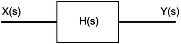
The Transfer Function (TF) of a System is the ratio of the output to the input of a system, in the Laplace domain considering its initial conditions and equilibrium point to be zero.

If we have an input function of X(s), and an output function Y(s), we define the transfer function H(s).

Impulse Response

Since we know that in the time domain, generally, we define the input to a system as x(t) and the output of the system as y(t). The relationship between the input and the output is represented as the impulse response, h(t) for the input as an impulse signal.

We can use the following equation to define the impulse response:

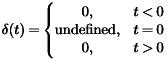
• The Impulse Function, denoted with δ(t) is a function defined piece-wise as follows

• An examination of the impulse function shows that it is related to the unit-step function as follows

u(t)= ∫δ(t) or

• The impulse response (IR) must always satisfy the following condition, or else it is not a true impulse function

Convolution in Time Domain

If we have the system input and the impulse response of the system, we can calculate the system output using the convolution operation as such as

y(t)=h(t)∗x(t).

Time-Invariant System Response

If the system is time-invariant, then the general description of the system can be replaced by a convolution integral of the system’s impulse response and the system input.We can call this the convolution description of a system.

Convolution Theorem

• Convolution in the time domain turns into multiplication in the complex Laplace domain.
• Multiplication in the time domain turns into convolution in the complex Laplace domain.

L[f(t)∗g(t)]=F(s).G(s)

L[f(t).g(t)]=F(s)∗G(s)

Result: If the complex Laplace variable is s, then we generally denote the transfer function of a system as either G(s) or H(s). If the system input is X(s), and the system output is Y(s), then the transfer function can be defined as such

• So if we know the input to a given system, and we have the transfer function of the system, we can solve for the system output by multiplying as

Y(s)=H(s).X(s)

Example: Impulse Response

• Since we know that the Laplace transform of the impulse function, δ(t) is L[δ(t)]=1
• So, when we put this into the relationship between the input, output, and transfer function, we get

Y(s)=X(s).H(s)

or Y(s)=(1).H(s)

or Y(s)=H(s)

In other words, the impulse response is the o/p of the system when we input an impulse function.

Transfer Functions for Linear Systems

Consider a linear input/output system described by the controlled differential equation

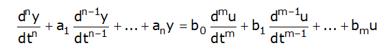
where u is the input and y is the output.

• To obtain the transfer function of the system of the last equation, let us take the input to be u(t) = e^st.
• Since the system is linear, there is an output of the system that is also an exponential function ⇒ y(t) = Y_oe^st.
• Inserting the signals into last equation ,we find

(sⁿ +a₁sⁿ⁻¹ +···+a_n)y_o.e^st = (b_os^m +b₁s^m−1···+b_m)e^−st

• And the response of the system can be completely described as

a(s) = sⁿ +a₁sⁿ⁻¹ +···+aⁿ & b(s) = b_os^m +b₁s^m−1 +···+b^m

• So, the transfer function of the given function is given by

Transfer Function Alternative Method

To investigate how a linear system responds to the exponential input u(t) = e^st we consider the state space system

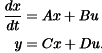
Let the input signal be u(t) = e^st and assume that s ≠ λ_i(A), where i = 1,2,3,…,n, where λ_i(A) is the ith eigenvalue of A. then

Since s ≠ λ(A) the integral can be evaluated and we get

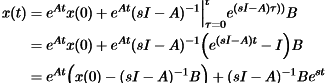
& Output y(t) = Cx(t) + Du(t)

= Ce^At{x(0)−(sI −A)⁻¹B}+[D+C(sI−A)⁻¹B]e^st

Note: One term of the output is proportional to the input u(t) = e^st. This term is called the pure exponential response.

• If the initial state is chosen as x(0) = (sI −A)⁻¹B
• the output only consists of the only exponential response and both the state and the output are directly proportional to the input

x(t) = (sI −A)⁻¹Be^st = (sI −A)⁻¹Bu(t)

y(t) = [C(sI −A)⁻¹B+D]e^st = [C(sI−A)⁻¹B+D]u(t).

• The ratio of the output and the input

G(s) = C(sI −A)⁻¹B +D is the transfer function of the system.

• For Homogeneous Equation i.e; D=0 then

G(s) = C(sI −A)⁻¹B is the transfer function of the system.

The Concept of Pole & Zero

• Poles and Zeros of a transfer function are the frequencies for which the value of the transfer function becomes infinity or zero respectively.
• The transfer function has many useful explanations and the features of a transfer function are often associated with important system properties. Three of the most important features are the gain and the locations of the poles and zeros.

• In the above equation, N(s) and D(s) are simple polynomials in s. Zeros are the roots of N(s) by setting N(s)=0 and solving for s. Poles are the roots of D(s), by setting D(s)=0 and solving for s.
• In general Transfer Function must not have more zeros than poles, we can state that the polynomial order of D(s) must be greater than or equal to the polynomial order of N(s).

Effects of Poles and Zeros

• when s approaches a zero (Zeros of Transfer function), the numerator of the transfer function N(s)→0.
• When s approaches a pole (Poles of Transfer Function), the denominator of the transfer function D(s)→0 &the value of the transfer function approaches infinity.
• An output value of infinity should raise an alarm bell for people who are familiar with BIBO stability.
• Poles & Zeros of a transfer function are represented in s-Plane, In s-plane s = σ±jω where σ represent the attenuation on X-axis & ω represents the angular velocity represented on the y-axis.
• In the s-plane, the Poles are located by a cross (*) & the Zeros are located by dot (.)

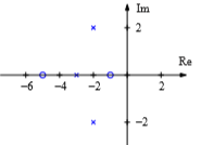
• For a Stable System, All the Poles & Zeros of a Transfer Function must be lie in the left half of the s-plane.

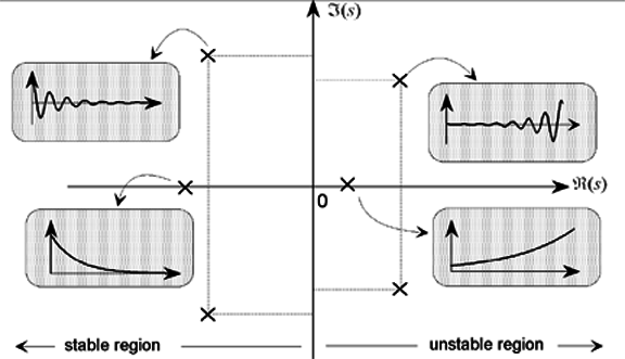
Note: If the Poles or Zero lie on the imaginary axis then it must be simple (order only 1) then the system is said to be Marginally Stable, If the Order of multiplicity of Poles or Zeros on Imaginary Axis is more than 1 in that case system will become Unstable.

Download Formulas for GATE Electrical Engineering – Electrical Machines PDF

If you are preparing for GATE and ESE, avail Online Classroom Program to get unlimited access to all the live structured courses and mock tests from the following link:

Online Classroom Program

BYJU’S Exam Prep Test Series