Signals & Systems : L.T.I. Systems

Linear systems have the property that the output is linearly related to the input. Changing the input in a linear way will change the output in the same linear way. So if the input x₁(t) produces the output y₁(t) and the input x₂(t) produces the output y₂(t), then linear combinations of those inputs will produce linear combinations of those outputs. The input {x₁(t)+x₂(t)} will produce the output {y₁(t)+y₂(t)}. Further, the input {a₁x₁(t)+a₂x₂(t)} will produce the output {a₁y₁(t)+a₂y₂(t)} for some constants a₁ and a₂.

In other words, for a system T over time t, composed of signals x₁(t) and x₂(t) with outputs y₁(t) and y₂(t) ,

Homogeneity Principle: 

Superposition Principle:

Thus, the entirety of an LTI system can be described by a single function called its impulse response. This function exists in the time domain of the system. For an arbitrary input, the output of an LTI system is the convolution of the input signal with the system's impulse response.

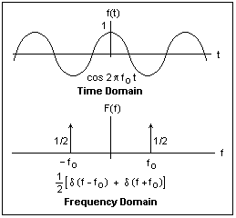
Conversely, the LTI system can also be described by its transfer function. The transfer function is the Laplace transform of the impulse response. This transformation changes the function from the time domain to the frequency domain. This transformation is important because it turns differential equations into algebraic equations, and turns convolution into multiplication.

In the frequency domain, the output is the product of the transfer function with the transformed input. The shift from time to frequency is illustrated in the following image:

Homogeneity, additivity, and shift-invariance may, at first, sound a bit abstract but they are very useful. To characterize a shift-invariant linear system, we need to measure only one thing: the way
the system responds to a unit impulse. This response is called the impulse response function of the system. Once we’ve measured this function, we can (in principle) predict how the system will
respond to any other possible stimulus.

Introduction to Convolution

Because here’s not a single answer to define what is? In “Signals and Systems” probably we saw convolution in connection with Linear Time-Invariant Systems and the impulse response for such a system. This multitude of interpretations and applications is somewhat like the situation with the definite integral.

To pursue the analogy with the integral, in pretty much all applications of the integral there is a general method at work:

• Cut the problem into small pieces where it can be solved approximately.
• Sum up the solution for the pieces, and pass to a limit.

Convolution Theorem

F(g∗f)(s)=Fg(s)Ff(s)

• In other notation: If f(t)⇔ F(s)  and g(t) ⇔ G(s) then (g∗f)(t)⇔ G(s)F(s)
• In words: Convolution in the time domain corresponds to multiplication in the frequency domain.

• For the Integral to make sense i.e., to be able to evaluate g(t−x) at points outside the interval from 0 to 1, we need to assume that g is periodic. it is not the issue the present case, where we assume that f(t) and g(t) are defined for all t, so the factors in the integral

Convolution in the Frequency Domain

• In Frequency Domain convolution theorem states that

F(g ∗ f)=Fg ·Ff

• here we have seen that the whole thing is carried out for inverse Fourier transform, as follow:

F⁻¹(g∗f)=F⁻¹g·F⁻¹f

F(gf)(s)=(Fg∗Ff)(s)

• Multiplication in the time domain corresponds to convolution in the frequency domain.

     By applying Duality Formula

     F(Ff)(s)=f(−s) or F(Ff)=f⁻   without the variable.

• To derive the identity  F(gf) = Fg∗Ff,  we assume for convenience, h = Ff and k = Fg

then we can write as     F(gf)=k∗h

• The one thing we know is how to take the Fourier transform of a convolution, so, in the present notation, F(k∗h)=(Fk)(Fh).

         But now       Fk =FFg = g⁻

         and likewise   Fh =FFf = f

         So F(k∗h)=g⁻f⁻ =(gf)⁻, or   gf =F(k∗h)⁻

        Now, finally, take the Fourier transform of both sides of this last equation 

        FF identity : F(gf)=F(F(k∗h)−)=k∗h =Fg∗Ff 

Note: Here we are trying to prove F(gf)(s) = (Fg∗Ff)(s) rather than F(g∗f)=(Ff)(Fg) Because, it seems more “natural” to multiply signals in the time domain and see what effect this has in the frequency domain, so why not work with F(fg) directly? But write the integral for F(gf); there’s nothing you can do with it to get toward Fg∗Ff. 

There is also often a general method of convolutions:

• Usually there’s something that has to do with smoothing and averaging,understood broadly.
• You see this in both the continuous case  and the discrete case.

Some of you who have seen convolution in earlier courses,you’ve probably heard the expression “flip and drag”

Meaning of Flip & Drag: here’s the meaning of Flip & Drag is as follow

• Fix a value t.The graph of the function g(x−t) has the same shape as g(x) but shifted to the right by t. Then forming g(t − x) flips the graph (left-right) about the line x = t.
• If the most interesting or important features of g(x) are near x = 0, e.g., if it’s sharply peaked there, then those features are shifted to x = t for the function g(t − x) (but there’s the extra “flip” to keep in mind).Multiply  f(x) and g(t − x) and integrate with respect to x.

Averaging

• I prefer to think of the convolution operation as using one function to smooth and average the other. Say g is used to smooth f in g∗f. In many common applications g(x) is a positive function, concentrated near 0, with total area 1.    

• Like a sharply peaked Gaussian, for example (stay tuned). Then g(t−x) is concentrated near t and still has area 1. For a fixed t, forming the integral

• The last expression is like  a weighted average of the values of f(x) near x = t, weighted by the values of (the flipped and shifted) g. That’s the averaging part of  the convolution, computing the convolution g∗f at t replaces the value f(t) by a weighted average of the values of f near t.

Smoothing  

• Again take the case of an averaging-type function g(t), as above. At a given value of t,( g ∗ f)(t) is a weighted average of values of f near t.
• Then Move t a little to a point t₀. Then (g∗f)(t₀) is a weighted average of values of f near t₀, which will include values of f that entered into the average near t.
• Thus the values of the convolutions (g∗f)(t) and (g∗f)(t₀) will likely be closer to each other than are the values f(t) and f(t₀). That is, (g ∗f)(t) is “smoothing” f as t varies — there’s less of a change between values of the convolution than between values of f.

Other identities of Convolution

It’s not hard to combine the various rules we have and develop an algebra of convolutions. Such identities can be of great use — it beats calculating integrals. Here’s an assortment. (Lower and uppercase letters are Fourier pairs.)

• (f ·g)∗(h·k)(t) ⇔ (F ∗G)·(H ∗K)(s)
• {(f(t)+g(t))·(h(t)+k(t)} ⇔ {[(F + G)∗(H + K)]}(s)
• f(t)·(g∗h)(t) ⇔ F ∗(G·H)(s)

Properties of Convolution

Here we are explaining the properties of convolution in both continuous and discrete domain

• Associative
• Commutative
• Distributive properties
• As a LTI system is completely specified by its impulse response, we look into the conditions on the impulse response for the LTI system to obey properties like memory, stability, invertibility, and causality.
• According to the Convolution theorem in Continuous & Discrete time as follow:

 For Discrete system .

  For Continuous System 

     We shall now discuss the important properties of convolution for LTI systems.

1) Commutative property :

• In Discrete time:    x[n]*h[n] ⇔  h[n]*x[n]

         Proof: Since we know that y[n] = x[n]*h[n]  

          Let us assume n-k = l   so,   

• So it clear from the derived expression that ⇒    x[n]*h[n] ⇔  h[n]*x[n]
• In Continuous time: 

         Proof

        So x[t]*h[t] ⇔ h[t]*x[t]

 2. Distributive Property

     By this Property we will conclude that convolution is distributive over addition.

• Discrete time:        x[n]{α h₁[n] + βh₂[n]} = α {x[n] h₁[n]}+ β{x[n] h₂[n]}        α & β are constant.
• Continuous Time:     x(t){α h₁(t) + βh₂(t)} = α{x(t)h₁(t)} + β {x(t)h₂(t)}            α & β are constant.

3. Associative Property

• Discrete Time  y[n] = x[n]*h[n]*g[n]

        x[n] * h₁[n] * h₂[n] = x[n] * (h₁[n] * h₂[n])

• In Continuous Time:

       [x(t) * h₁(t)] * h₂(t) = x(t) * [h₁(t) * h₂(t)]

       If systems are connected in cascade:

∴ Overall impulse response of the system is:

 4. Invertibility

 A system is said to be invertible if there exist an inverse system which when connected in series with the original system produces an output identical to input .

     (x*δ)[n]= x[n]

     (x*h*h^-1)[n]= x[n]

     (h*h^-1)[n]= (δ)[n]

5. Causality

• Discrete Time

• Continuous Time 

 6. Stability

• Discrete Time

• Continuous Time

You can avail of BYJU’S Exam Prep Online classroom program for all AE & JE Exams:

BYJU’S Exam Prep Online Classroom Program for AE & JE Exams (12+ Structured LIVE Courses)

You can avail of BYJU’S Exam Prep Test series specially designed for all AE & JE Exams:

BYJU’S Exam Prep Test Series AE & JE Get Unlimited Access to all (160+ Mock Tests)

Thanks

Team BYJU’S Exam Prep

Download  BYJU’S Exam Prep APP, for the best Exam Preparation, Free Mock tests, Live Classes.