Control Systems : Various Plots

Bode Plot

The bode plot gives a graphical method for determining the stability of a control system based on sinusoidal frequency response. Bode graphs are representations of the magnitude and phase of G(j*ω) (where the frequency vector ω contains only positive frequencies).

The bode plot consists of two graphs: Magnitude plot and Phase plot

• 20 log₁₀ |G (jω)| versus logω, this is called the magnitude plot.
• Phase shift (in degrees) versus logω (frequency), is called phase plot.
• Bode plots are asymptotic log magnitude and phase plots. These are drawn as straight lines.
• The corner frequency is the frequency at which the slope of the asymptotic log magnitude plot changes.
• The frequency band from ω₁ and ω₂ such that (ω₂/ω₁) = 10 is called a decade.
• For a first-order factor, the slope of the Log magnitude plot changes by ±20 dB/decade at the corner frequency according to as the factor is in the numerator or denominator respectively. For a second-order factor, the slope changes by ±40 dB/decade and so on.

Initial Slope of the Bode Plot: Initial slope can be determined by the type of the system, Its value is different for different types of system.

• Type 0 system: For this system, the initial slope is 0 dB/decade with dB value 20 log K.

• Type 1 system: For this system, the initial part of the system is

• Type 2 system: For type 2 system, the initial part of the plot is

Here, the initial slope is -40 dB/decade and plot cuts the 0 dB line at 

Phase Margin and Gain Margin

The PM and GM can be calculated by considering the following plot

• Gain Crossover Frequency: Frequency at which magnitude plot crosses the 0 dB line.
• Phase Crossover Frequency: Frequency at which phase plot crosses the -180° line
• Gain Margin: Value of gain from gain plot at phase crossover frequency is called gain margin. Gain margin is positive if it is below zero dB line
• Phase Margin: Value of phase from phase plot at the gain crossover frequency is known as phase margin. Phase margin is positive if it is above -180° line

Minimum Phase, Non-minimum Phase and All Pass Transfer Function

• Minimum phase transfer function: 

• Non-minimum phase system: 

• All pass transfer functions: 

• If there are no poles of the transfer function at the origin, the initial slope of the LM plot is zero and the magnitude is 20 log K_p up to the lowest corner frequency.
• If there is a single pole at the origin of the open loop transfer function the LM plot has an initial slope equal to -20 dB/decade up to the lowest corner frequency and if this line is extended, it will intersect the frequency axis at ω = k_v.
• If there are two poles at the origin of the open loop transfer function, the LM plot has an initial slope equal to -40 dB/decade up to the lowest corner frequency and this line is extended will intersect the frequency axis at .
• If there is one zero at the origin, the LM plot has an initial slope equal to 20 dB/decade up to the lowest corner frequency. If there are two zeros at the origin, the LM plot has an initial slope equal to +40 dB/decade up to the lowest corner frequency and so on
• Multiplication of the transfer function by a gain factor is equivalent to shifting the LM plot vertically up by an equivalent gain in dB.

Effects of Addition of Poles: The effects of addition of poles are as follows

• There is change in shape of the root locus and it shifts towards the imaginary axis. The intercept on the jω axis occurs for a lower value of K because of asymptote angle being lower down.
• System becomes oscillatory.
• Gain margin and relative stability decrease.
• There is reduction in the range of K.
• A sluggish response can be changed to a quicker response for the artful introduction of a pole.
• Settling time increases.

Effects of Addition of Zeros: The effects of addition of zeros are as follows

• There is change in shape of the root locus and it shifts towards the left of the s-plane.
• Stability of the system is enhanced.
• Range of K increases.
• Settling time speeds up.

Polar Plot

The polar plot of a sinusoidal transfer function G(jω) is a plot of the magnitude of G(jω) versus the phase angle of G(jω) on polar coordinates as ω varied from zero to infinity.

Procedure to Sketch the Polar Plot:

• Step-1: Determine transfer function G(jω).
• Step-2: Put s = jω in the transfer function to obtain G(jω).
• Step-3: At ω = 0 and m = ∞, calculate | G(jω)| by  and .
• Step-4: Calculate the phase angle of G(jω) at ω = 0 and ω = ∞ by  and .
• Step-5: Rationalize the function G(jω) and separate the real and imaginary axis.
• Step-6: Equate the imaginary part Im|G(jω)| to zero and determine the frequencies at which plot intersects the real axis and calculate the value of G(jω) at the point of intersection by substituting the determined value of frequency in the expression of G(jω).
• Step-7: Equate the real part Re|G(jω)| to zero and determine the frequencies at which plots intersects the imaginary axis and calculate the value G(jω) at the point of intersection by substituting the determined value of frequency in the rationalized expression of G(jω).
• Step-8: Sketch the polar plot with the help of the above information.

Polar Plot of Some Standard Functions:

• Type 0 System 

• Type 1 System

• Type 2 System

Introduction of Additional Pole

Polar Plot for 

Polar Plot For 

Gain Margin and Phase Margin with Polar Plot

• Phase Crossover Frequency: The frequency at which the polar plot crosses the -180° line is called the phase crossover frequency.
• Gain Crossover Frequency: The frequency at which the polar plot crosses the unit circle is called gain crossover frequency.
• Gain Margin: At phase crossover frequency, if the gain is 'a' then

Gain margin = - 20 log a

• Phase Margin (φ_m): At gain crossover frequency, if the phase is φ then phase margin

φ_m = 180 + φ

       where, φ is positive from anti-clockwise direction.

Nyquist Stability Criterion

A stability test for time-invariant linear systems can also be derived in the frequency domain. It is known as the Nyquist stability criterion. It is based on the complex analysis result known as Cauchy’s principle of argument. Nyquist criterion is used to identify the presence of roots of a characteristic equation of a control system in a specified region of the s-plane. The nyquist approach is the same as Routh-Hurwitz but, it differs with the following aspect:-

• The open loop transfer function "G(s)H(s)" is considered instead of closed loop characteristic equation " 1+G(s) H(s) = 0".
• Inspection of the graphical plot of G(s) H(s) enables to get more than yes or no answer of Routh-Hurwitz method pertaining to the stability of control system.
• Nyquist plots display both amplitude and phase angle on a single plot, using frequency as a parameter in the plot.
• Nyquist plots have properties that allow you to see whether a system is stable or unstable. It will take some mathematical development to see that, but it's the most useful property of Nyquist plots.

Concept of Encirclement & Enclosement

Encirclement:

• point A is encircled in the counter in Counter Clock Wise by closed path, while point B is NOT encircled by closed path.

Enclosement: A point or region is said to be enclosed by a closed path if the point or region lies to the right of the path when the path is traversed in any prescribed direction.

• In figure (a) point A is not enclosed by the path, while Point B is enclosed by the path.
• In figure (b) point A is enclosed by the path, while point B is not enclosed by the path.

Nyquist Stability Criterion: Fundamentals

Consider the phasor from point A to S₁ of encirclement = N, the net angle traversed by the phasor = 2πN rad

• In figure (a) Point A of encirclement = +1; Point B of encirclement = +2.
• In figure (b) Point A of encirclement = -1; Point B of encirclement = -2.

Determination of N:

• For a SISO feedback system, the closed-loop transfer function is given by

• closed-loop system poles are obtained by solving the following equation

       1+G(s)H(s) =0 =Δ(s) represents the system characteristic equation.

• In the following, we consider the complex function

D(s) = 1+G(s)H(s)

• The zeros of D(s) are the closed-loop poles of the transfer function. Here now we concluded that the poles of D(s) are the zeros of M(s).
• At the same time, the poles of D(s) are the open-loop control system poles since they are contributed by the poles of H(s)G(s), which can be considered as the open-loop control system transfer function—obtained when the feedback loop is open at some point.
• The Nyquist stability test is obtained by applying the Cauchy principle of argument to the complex function D(s). First, we state Cauchy’s principle of argument.

Cauchy’s Principle of Argument

• Let F(s) be an analytic function in a closed region of the complex s-plane, except at a finite number of points (namely, the poles of F(s)).
• It is also assumed that F(s) is analytic at every point on the contour. Then, as 's' travels around the contour in the s-plane in the clockwise direction, the function F(s) encircles the origin in the [ReF{(s)}, Img{F(s)}]-plane in the same direction N times, where N is given By

N= P-Z

       where Z and P stand for the number of zeros and poles (including their multiplicities) of the function F(s) inside the contour.

• The above result can be also written as 

arg{F(s)} = (Z-P)2π = 2Nπ

Nyquist Plot

The Nyquist plot is a polar plot of the function D(s) = 1+ G(s)H(s) when travels around the contour

• The contour in the above figure covers the whole unstable half-plane of the complex plane s, R→∞.
• Since the function D(s), according to Cauchy’s principle of argument, must be analytic at every point on the contour, the poles D(s) of on the imaginary axis must be encircled by
  infinitesimally small semicircles.

Nyquist Criterion: 

• It states that the number of unstable closed-loop poles is equal to the number of unstable open-loop poles plus the number of encirclements of the origin of the Nyquist plot of the complex function F(s).
• The above criterion can be slightly simplified if instead of plotting the function "D(s) = 1+G(s)H(s)", we plot only the function G(s)H(s) and count encirclement of the Nyquist plot of G(s)H(s) around the point (-1+j0). 
• The number of unstable closed-loop poles (Z) is equal to the number of unstable open-loop poles (P) plus the number of encirclements (N) of the point (-1+j0) of the Nyquist plot of G(s)H(s), that is

Z= P+N

Phase and Gain Stability Margins

Two important notions can be derived from the Nyquist diagram: phase and gain stability margins. The phase and gain stability margins are presented in the Figure below

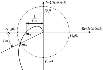
• They give the degree of relative stability; in other words, they tell how far the given system is from the instability region. Their formal definitions are given by

• where ω_gc and ω_pc stand for, respectively, the gain and phase crossover frequencies, which are obtained from the figure as 

Example: Consider a control system represented by

Solution: Since this system has a pole at the origin, the contour in the -plane should encircle it with a semicircle of an infinitesimally small radius. This contour has three parts (a), (b), and (c). Mappings for each of them are considered below.

•  On this semicircle, the complex variable 's' is represented in the polar form by 's = Re^jψ' with R→∞, - π/2 ≤ ψ ≥ π/2. Substituting 's = Re^jψ' into G(s)H(s), we easily see that G(s)H(s)→0. Thus, the huge semicircle from the -plane maps into the origin in the -plane.

         Thus, the huge semicircle from the s-plane maps into the origin in the G(s)H(s)-plane.

• On this semicircle, the complex variable is represented in the polar form by 's = re^jψ' with r→0, - π/2 ≤ ψ ≥ π/2. so that we have

     Since φ changes from  '- π/2' at point A to ' π/2' at point B, arg{G(s)H(s)} will change from "π/2 to -π/2". We conclude that the infinitesimally small semicircle at the origin in the s-plane is mapped into a semicircle of infinite radius in the G(s)H(s)-plane.

• On this part of the contour, s takes pure imaginary values, i.e.  s= jω with ω  changing from'-∞ to +∞'.Due to symmetry, it is sufficient to study only mapping along "0⁺≤ ω ≥+∞". We can find the real and imaginary parts of the function G(jω)H(jω), which are given by

From the above expressions, we see that neither the real nor the imaginary parts can be made zero, and hence the Nyquist plot has no points of intersection with the coordinate axis. For ω= 0⁺ we are at point B and since the plot at  ω= +∞ will end up at the origin. Note that the vertical asymptote of the Nyquist plot is given by

{Re G(jo±)H(jo±)} = -1

• From the Nyquist diagram we see that N= 0 and since there are no open-loop poles in the left half of the complex plane, i.e.P=0, we have Z =0 so that the corresponding closed-loop system has no unstable poles.