Probability & Distributions

Probability Distributions

Probability Distributions are fundamental concepts in the field of mathematics, playing a crucial role in understanding and analyzing uncertainties and random phenomena. These concepts provide a framework for quantifying the likelihood of events and outcomes, and for describing the behavior and characteristics of random variables. Engineers and mathematicians rely on probability theory and distributions to make informed decisions, assess risk, design experiments, analyze data, and develop accurate mathematical models. With wide-ranging applications in various fields, Probability Distributions form the bedrock of problem-solving and decision-making processes, enabling a deeper understanding of complex systems and phenomena.

Combinatorial Analysis

To have an understanding of combinations and permutations you must first have a basic understanding of probability.A probability is a numerical measure of the likelihood of the event. Probability is established on a scale from 0 to 1. A rare event has a probability close to 0; a very common event has a probability close to 1.

In order to solve and understand problems pertaining to probability you must know some vocabulary:

• An experiment, such as rolling a die or tossing a coin, is a set of trials designed to study a physical occurrence.
• An outcome is any result of a particular experiment. For example, the possible outcomes for flipping a coin are heads or tails.
• A sample space is a list of all the possible outcomes of an experiment.
• An event is a subset of the sample space. For example, getting heads is an event.

Counting Principles

1. Theorem (The basic principle of counting): If the set E contains n elements and the set F contains m elements, there are nm ways in which we can choose, first, an element of E and then an element of F.
2. Theorem (The generalized basic principle of counting): If r experiments that are to be performed are such that the first one may result in any of n1 possible outcomes, and if for each of these n1 possible outcomes, there are n2 possible outcomes of the second experiment, and if for each of the possible outcomes of the first two experiments, there are n3 possible outcomes of the third experiment, and if …, then there is a total of n­1.n2…nr, possible outcomes of the r experiments.
3. Theorem: A set with n elements has 2n subsets.
4. Tree diagrams

Permutations

1. Permutation: n!
   The number of permutations of n things taken r at a time:
2. Theorem: The number of distinguishable permutations of n objects of k different types, where n1 are alike, n2 are alike, …, nk are alike and n=n1+n2+…+nk, is

Combinations

1. Combination: The number of combinations of n things taken r at a time: (combinatorial coefficient; binomial coefficient)
2. Binomial theorem:
3. Multinomial expansion: In the expansion of (x1+x2+…+xk)n, the coefficient of the term , n1+n2+…+nk=n, is . Therefore, (x1+x2+…+xk)n = .
   Note that the sum is taken over all nonnegative integers n1, n2,…,nk such that n1+n2+…+nk=n.

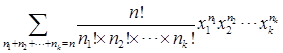
The Number of Integer Solutions of Equations

1. There are distinct positive integer-valued vectors (x1,x2,…,xy) satisfying x1+x2+…+xr = n, xi>0, i=1,2,…,r.
2. There are distinct nonnegative integer-valued vectors (x1,x2,…,xy) satisfying x1+x2+…+xr = n.

Axioms of Probability

The Axioms of Probability are foundational principles that define the rules and properties of probability theory. These axioms provide a rigorous framework for quantifying and reasoning about uncertainty and likelihood in mathematical and statistical contexts.

Sample Space and Events

1. Experiment: An experiment (strictly speaking, a random experiment) is an operation which can result in two or more ways. The possible results of the experiment are known as the outcomes of the experiment. These outcomes are known in advance. We cannot predict which of these possible outcomes will appear when the experiment is done.
2. Sample Space: The set containing all the possible outcomes of an experiment as its element is known as sample space. It is usually denoted by S.
3. Event: An event is a subset of the sample space S.

Illustration 1:

Let us consider the experiment of tossing a coin. This experiment has two possible outcomes: heads (H) or tails (T)

• sample space (S) = {H, T}

We can define one or more events based on this experiment. Let us define the two events A and B as:

A: heads appears

B: tails appears

It is easily seen that set A (corresponding to event A) contains outcomes that are favourable to event A and set B contains outcomes favourable to event B. Recalling that n (A) represents the number of elements in set A, we can observe that

n (A) = number of outcomes favourable to event A

n (B) = number of outcomes favourable to event B

n (S) = number of possible outcomes

Here, in this example, n (A) = 1, n (B) = 1, and n (S) = 2.

• Set theory concepts: set, element, roster method, rule method, subset, null set (empty set).
• Complement: The complement of an event A with respect to S is the subset of all elements of S that are not in A. We denote the complement of A by the symbol A’ (Ac).
• Intersection: The intersection of two events A and B, denoted by the symbol A∩B, is the event containing all elements that are common to A and B.
  Two events A and B are mutually exclusive, or disjoint, if A∩B = φ that is, if A and B have no elements in common.
• The union of the two events A and B, denoted by the symbol A∪B, is the event containing all the elements that belong to A or B or both.

• Venn diagram:
• Sample space of an experiment: All possible outcomes (points)
• Events: subsets of the sample space
  Impossible events (impossibility): Φ; sure events (certainty): S.

• DeMorgan’s laws:

Axioms of Probability

1. Probability axioms:
   (1) 0≤P(A)≤1;
   (2) P(S)=1;
   (3) P(A1∪A2∪…) = P(A1)+P(A2)+… If {A1, A2, …} is a sequence of mutually exclusive events.
2. Equally likely outcomes: the probabilities of the single-element events are all equal.
   A number of sample events are said to be equally likely if there is no reason for one event to occur in preference to any other event.

Basic Theorems

(1) 0≤P(A)≤1;

(2)

(3) Complementary events:

(4) P(A∪B) = P(A) + P(B) – P(A∩B): inclusion-exclusion principle

(5) If A1, A2, An is a partition of sample space S, then

(6) if a and a’ are complementary events, then P(A) + P(A’)=1.

Conditional Probability and Independence

Conditional Probability and Independence are important concepts in probability theory. Conditional probability measures the likelihood of an event occurring given that another event has already happened, while independence describes the absence of a relationship between two events.

Conditional Probability

1. Conditional probability:

Consider two events A and B defined on a sample space S. The probability of occurrence of event A given that event B has already occurred is known as the conditional probability of A relative to B.

P(A/B) = P(A given B) = probability of occurrence of A assuming that B has occurred

It implies that the outcomes favourable to B become the possible outcomes and hence outcomes favourable to P(A/B) are outcomes common to A and B.

Let n(B)=a and n(A∩B)=b. Suppose that event B occurs. Then there are exactly sample points and these points can be considered to be the sample space for the other event A. Event A in this sample space consists of b sample points common to A and B.

Therefore, the probability of A in this sample space = b/a.

Thus the probability of A under the assumption that event B has occurred is:

and similarly

The above result is known as the conditional probability theorem.

2. If in an experiment the events A and B can both occur, then P(A∩B) = P(A)P(B|A) = P(B)P(A|B).

P(A∩B∩C) = P(A∩B)P(C|A∩B) = P(A)P(B|A)P(C|A∩B),

The multiplication rule: P(A1∩A2 ∩…∩ An) = P(A1)P(A2|A1)P(A3|A1∩A2) … P(An|A1∩A2∩…∩An-1).

3. Partition: Let {B1, B2, …, Bn} be a set of nonempty subsets of the sample space S of an experiment. If the events B1, B2, …, Bn are mutually exclusive and B1∪B2∪…∪Bn = S, the set {B1, B2, …, Bn} is called a partition of S.

4. Theorem of total probability: If B1, B2, … is a partition of S, and A is any event, then

Total Probability Theorem: The probability that one of several mutually exclusive events A1, A2, .... An will happen is the sum of the probabilities of the separate events. i.e.

P(A1∪A2∪An) = P(A1)+P(A2)+.... + P(An)

5. Bayes’ Theorem: If B1, B2, … is a partition of S, and A is any event, then

Independence

1. Independent events: If A, B are independent events ↔ P(A∩B) = P(A)P(B).
2. Theorem: If A and B are independent, then are independent.
3. The events A, B, and C are called independent if P(A∩B) = P(A)P(B), P(A∩C) = P(A)P(C), P(B∩C) = P(B)P(C), P(A∩B∩C) = P(A)P(B)P(C). If A, B, and C are independent events, we say that {A, B, C} is an independent set of events.
4. The set of events {A1, A2, …, An} is called independent if for every subset of {A1, A2,…, An},.

Important Results

The following results are easily derived from the definition of independent events.

1. A and B are independent if
   P(B/A) = P(B) and P(A/B) = P(A)
2. If A and B are independent, then P (A∩B) = P (A) P (B)
3. A set of events A1, A2,... An is said to be pair-wise independent if
   P(Ai n Aj) = P(Ai) P(Aj) ∀i ≠j.
4. The events A1, A2, ... An are mutually independent (or simply independent) if and only if the multiplication rule:
   P(A1∩A2∩ .... Ak) = P(A1) P(A2) .... P(Ak) ... (1)
   holds for every t triples of events, k = 2, 3, .... n. If (1) holds for k = 2 and may not hold for k = 3, 4, ....... n then events A1, A2, ... An are said to be pairwise independent. Thus mutually independent events are pairwise independent but the converse is not true.
5. If A and B are mutually independent events such that P (A) ≠ 0 and P (B) ≠ 0, then the events A and B have at least one common sample point (i.e. they cannot be mutually exclusive). Or in general, mutually exclusive events are dependent events.

Distribution Functions and Discrete Random Variables

Distribution functions and discrete random variables are fundamental concepts in probability theory. Distribution functions describe the probability of obtaining specific outcomes in discrete random variables, providing a framework for analyzing and predicting their behaviour.

Distribution Functions

1. Cumulative Distribution Functions (cafe): FX(t) = P(X≤t), -∞ < t < ∞.

2. FX(t) is non-decreasing; 0≤FX(t)≤1;

If c<d, then FX(c)≤FX(d); P(c<X≤d) = FX(d)-FX(c); P(X>c) = 1-FX(c).

The cdf of a discrete random variable: a step function.

Special Discrete Distributions

Special Discrete Distributions are a set of probability distributions that are specifically tailored to model and analyze discrete random variables with distinct characteristics and unique applications in various fields.

Bernoulli and Binomial Random Variables

1. Bernoulli trials: an experiment with two different possible outcomes

Bernoulli random variable X with parameter p, p is the probability of success.

px(x) = px(1-p)1-x = pxq1-x, for x∈RX = {0,1}

Expected value: E[X] = μx = p; variance:

2. Binomial distribution: number of successes to occur in n repeated, independent Bernoulli trials

Binomial random variable Y with parameters n and p

Expected value: E(Y) = μY = np; Variance:

Multinomial Random Variables

1. Multinomial trials: an experiment with k≥2 different possible outcomes

2. Multinomial distribution: n independent multinomial trials

Multinomial random variable X1, X2, …, Xk with parameters n, p1, p2, …pk; Xt: the number of ith outcomes;;;

Geometric distribution: trial number of the first success to occur in a sequence of independent Bernoulli trials

Geometric random variable N with parameter p

Geometric series:

Expected value: ; variance:

Negative binomial distribution: trial number of the rth success to occur

Negative binomial random variable N, with parameters r, p

Expected value: ; variance:

Poisson Distribution

The Poisson Distribution is a probability distribution that models the number of events occurring within a fixed interval of time or space, often used to analyze rare or random events.

1. The Poisson probability function:

Poisson random variable K with parameterλ

Expected value: E(K) = μK = λ; variance:

2.the Poison approximation to the binomial: If X is a binomial random variable with parameters n and p=λ/n, then

Continuous Random Variables

Continuous random variables are a key concept in probability theory, representing variables that can take on an uncountable number of values within a specified range. They are essential for modelling real-world phenomena with continuous measurements, such as time, distance, and temperature.

Probability Density Functions

1. Densities

2. Probability density function (pdf) for a continuous random variable X: fx(x)

fx(x)≥0

For all

Cumulative Distribution Functions (CDF)

1.

2. The cdf of a discrete random variable: a step function; the cdf of a continuous random variable: a continuous function

3. The probability function of a discrete random variable: the size of the jump in FX(t); the pdf of a continuous random variable:

Expectations and Variances

1. Definition: If X is a continuous random variable with pdf fx(x), the expected value of X is defined by.

Example: In a group of adult males, the difference between the uric acid value and 6, the standard value, is a random variable X with the following pdf: fx(x) = (3x2 – 2x) if 2/3<x<3. Calculate the mean of these differences for the group.

2. Theorem: Let X be a continuous random variable with pdf fx(x); then for any function h:.

3. Corollary: Let X be a continuous random variable with pdf fx(x). Let h1, h2, …, hn be real-valued functions and α1, α2, …, αn be real numbers. Then E[α1h1(X) + α2h2(X) + … + αnhn(X)] = α1E[h1(X)] + α2E[h2(X)] + … + αnE[hn(X)].

4. Definition: If X is a continuous random variable with E[X] = μx, then Var[X] and σx, called the variance and standard deviation of X, respectively, are defined by , .

Special Continuous Distributions

Special Continuous Distributions encompass a set of probability distributions that are particularly useful in modelling and analyzing continuous random variables. These distributions have distinct characteristics and features, making them valuable tools in various fields such as statistics, engineering, and finance.

Uniform Random Variable

1. Density of a uniformly distributed random variable:

2. The cdf of a uniformly distributed random variable:

3. The expected value and variance of the uniform random variable: ; .

The Exponential Distribution

1. The exponential probability law with parameter λ:

T1 is the time of occurrence of the first event in a Poisson process with parameter λ, starting at an arbitrary origin t=0; {Xλt = 0} ≡ {T1>t}, Poisson process Xλt is the number of events to occur with parameter μ=λt.

2. The expected value and variance of the exponential random variable:

The Erlang Distribution

1. The cdf and pdf for T2:

T2 Is the time of occurrence of the second event in a Poisson process with parameter λ, starting at an arbitrary origin t=0; {Xλt ≤ 1} ≡ {T2>t}, Poisson process Xλt is the number of events to occur with parameter μ=λt?

2. The Erlang probability law with parameters r and λ:

Tr is the time of occurrence of the rth event in a Poisson process with parameter λ, starting at an arbitrary origin t=0; {Xλt ≤ r - 1} ≡ {Tr>t}, Xλt is the number of events to occur.

3. The expected value and variance of the Erlang random variable:

The Gamma Distribution

1. The gamma probability law with parameters n and λ: for u>0, n>0, λ>0.

Gamma function: ; Γ(n) = (n-1)Γ(n-1); Γ(n) = (n-1)!, if n is a positive integer.

The Erlang random variable is a particular case of a gamma random variable, where n is restricted to the integer values r=1,2,3,….

2. The expected value and variance of the gamma random variable:

The Normal (Gaussian) Distribution

1. The normal probability law with parameters μ and σ: , for -∞<x<∞,σ>0.

2. The expected value and variance of the normal random variable:.

3. Standard normal random variable (the unit normal): , μ=0, σ=1.

4. The new random variable: If X is normal with mean μ and variance σ2, then X+b is normal with mean μ+b and variance σ2; aX is normal with mean aμ and variance a2σ2; aX+b is normal with mean aμ+b and variance a2σ2.

5. Switching from a non-unit normal to the unit normal: , μz=0, σz=1.

6. The probability that a normal random variable is with k standard deviations of the mean: P(μ-kσ≤X≤μ+kσ) = P(-k≤X*≤k), X* is the unit normal.

7. The normal approximation to the binomial: A binomial distribution X with parameters n, p where n is large, then X is approximately normal with μ = np, σ2 = npq.

Jointly Distributed Random Variables

Jointly Distributed Random Variables are a fundamental concept in probability theory that involves the study of multiple random variables and their combined probability distributions.

Joint Densities

1. Jointly distributed random variable: If the observed values for two or more random variables are simultaneously determined by the same random mechanism.

2. The discrete random variables X1, X2: the probability function is for all x1, x2; . The continuous random variables X1, X2: the pdf is positive; for all x1, x2; ; the probability is given by integrating .

3. The joint density of independent random variables: The random variables X, Y are independent if and only if pX,Y(x,y) = pX(x)pY(y), when X, Y are discrete; fX,Y(x,y) = fX(x)fY(y), when X, Y are continuous.

4. Uniform joint densities: If X and Y are jointly uniformed on a region, the joint pdf is , for (x, y) in the region.

The joint density of independent uniform random variables:

Marginal Densities

1. The discrete random variables X1, X2 with the probability function and range , the marginal probability function for X1 is for is the marginal range for X1, the set of first elements of .

2. The continuous random variables X1, X2 with pdf and range , the marginal pdf for X1 is for . is the marginal range for X1, the set of first elements of .

Sums of Independent Random Variables

1. The sum of independent binomials with a common p: X1 with parameters n1, p, X2 with parameters n2, p, then X1+X2 with parameters n1+n2,p

2. The sum of independent Poissons: X1 with parameter λ1, X2 with parameters λ2, then X1+X2 with parameters λ1+λ2

3. The sum of independent exponentials with a common λ: X1, …, Xn with parameter λ, then X1 +…+ Xn has a gamma(Erlang) distribution with parameters n,λ.

4. The density of the sum of two arbitrary independent random variables: the convolution of the individual pdf,

5. The sum of independent normals: X1 with mean μ1 and variance with mean μ2 and variance , then X1+X2 with mean μ1+μ2 and variance

Get complete information about the GATE exam pattern, cut-off, and all those related things on the BYJU’S Exam Prep official youtube channel.

Daily free APP and Youtube classes, Engineering Jobs, Free PDF & much more, Join our Telegram Group Join Now.